Enable Data Connections Message Bar
When a pivot table is opened in Microsoft Excel the Message Bar will oftentimes display a Security Warning; these Security Warnings disable the connections to the data within the PivotTable. To override the security Warnings and enable the data connection each time the PivotTable is opened, simply select Enable Content in the Message Bar (A).
Analysis Services Cubes: Enable Content

Adding Measures to the PivotTable
What is a Measure or Value? A measure represents a column that contains quantifiable data, usually numeric, that can be aggregated.
The most fundamental part of a PivotTable is a Measure (Value). Examples of measures are Total Charges, Visit Counts, Average Cost, Etc. To add a measure to your PivotTable, use your left mouse button to drag a Measure (Value) from the Pivot Table Field List (A) down to Values (B). This will populate the row and column values within the report. (C)
Hint: Clicking the Value (B) in the Field list once will provide you access to the Value Field Set- tings where you can change the format of the Measure (Value) or change the way the Measure is displayed.

Adding PivotTable Rows
Using your left mouse button, drag an Attribute from the Pivot Table Field List (A) down to the
Row Labels (B). This will populate the rows within the report. (C)
Hint: You can apply a filter to a row in the report simply by using the drop down arrow on the left of the row header. (D) You can also add an attribute to your report by simply dragging the Attribute directly to the row area.

Adding PivotTable Columns
Using your left mouse button, drag an Attribute from the Pivot Table Field List (A) down to the
Column Labels (B). This will populate the columns within the report. (C)
Hint: You can apply a filter to a column in the report simply by using the drop down arrow on the left of the column header. (D) You can also add an attribute to your report by simply dragging the Attribute directly to the column area.

Adding PivotTable Filters
By default, PivotTables aggregate all Measures in the dataset; this can be many years of data which typically will need to be narrowed down. To focus on a smaller portion of a large amount of the PivotTable data for in-depth analysis, you can filter the data.
Applying a filter to the data while hiding it in the report
Using your left mouse button, drag an Attribute from the Pivot Table Field List (A) down to the Report Filters (B) and it will automatically show up as a report filter above the report. (C) The drop down arrow on the left of the filter allows you to select the years to be filtered.

Sorting Data
If you would like to order the Measures in the PivotTable simply select one of the values in the columns you would like to sort (A) and select the Sort and Filter option from the toolbar (B). There are two options, sort ascending (A to Z) or descending (Z to A).

Inserting a Chart
If you would like to add a dynamic PivotChart to your workbook, simply place your cursor on the data area you would like to chart. (A) Select the Insert menu option in the ribbon. (B) Select the type of chart you would like to create (Column, Line, Pie, Bar, or others). (C) This will create a dynamic chart that you can modify and move to other worksheets. (D)

Chart Hints
Right clicking on the bars on the chart will allow you to change colors, add data labels, change chart type, and add trend lines.

Analysis Services Cubes: Filter options
The filter options within the chart are dynamic; this will allow you to continue to manipulate the data in the chart simply by clicking the drop down arrow and changing the filter.

Analysis Services Cubes: Right clicking on an axis
Right clicking directly on an axis will allow you to change the formatting of the axis. (i.e. change the axis labels to show the values as currency)

Analysis Services Cubes: Layout Ribbon
Selecting the chart provides you with access to the Layout ribbon. This ribbon allows you access to a wide variety of functions such as add chart titles, change axis titles, altering the location of the legend, and modifying gridlines.

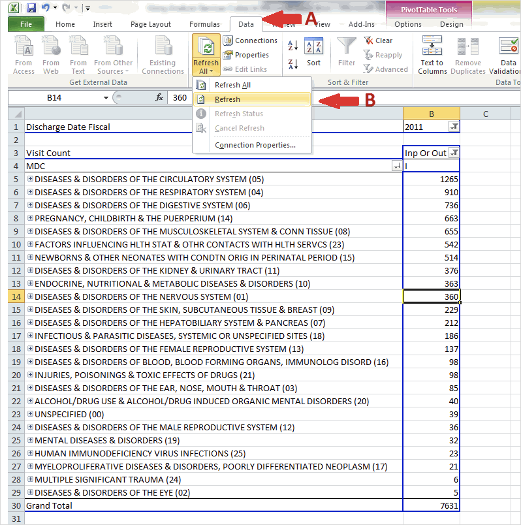
Refreshing Data
The PivotTable maintains a link back to the SQL Server Analysis Services cubes. Each night, when the RAPID datamart is updated these cubes are also updated. To refresh your PivotTable with the new data, select the Data menu in the ribbon (A), select Refresh All then Refresh (B).
Saving PivotTable in Excel Format
To save your PivotTable select File then Save As. (A) When the Save As dialogue box is opened, change the Save As Type to Excel Workbook (B).

Storing the Excel PivotTable in RAPID
Many users may want to store the PivotTable on a private or network drive. Others may want to store the table back into RAPID. To store the PivotTable back into RAPID, navigate to the module within RAPID where you would like the PivotTable to be stored. Open the Ad Hoc tab and select Embed File (A).

In the Embed File dialogue box populate the Name of the file. This is the name that will be displayed in RAPID; it can be different than the name of the Excel workbook. Select Browse to navigate to the location of the Excel PivotTable workbook, and click Embed File.

Troubleshooting
Q: What if the field list is no longer display? How do I get it back?
A: If your field list disappears and you would like to display it again there are two ways to make it visible again:
- Right Click anywhere inside of the pivot table and select Show Field List in the option box (A).
- Select Options (B) in the ribbon menu and select Field List (C)

Q: It seems that there is some data missing in the pivot table? How do I refresh the data?
A: If your pivot table does not appear to have the most recent data you may need to refresh the pivot table. There is a link between Excel and the Cube and refreshing the pivot table will pull in the latest data. There are two ways to “Refresh” the pivot table:
- Right Click anywhere inside of the pivot table and select Refresh in the option box (A).
- Select Options (B) in the ribbon menu and select Refresh All (B).
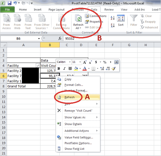
Hint: You can also refresh your data by simply right clicking in the middle of the PivotTable and select refresh. If you would like the data to refresh automatically, change the settings in Data -> Connections -> Properties -> Refresh when opening the file.